Land Cover Mapping - Part 1
Published on May 31, 2020 | Bikesh Bade | 5412 Views
The surface of the Earth is continuously changing at many levels; local, regional, national, and global scales. Changes in land use and land cover are pervasive, rapid, and can have significant impacts on people, the economy, and the environment. Land cover maps represent spatial information on different types (classes) of physical coverage of the Earth's surface, e.g. forests, grasslands, croplands, lakes, wetlands, snow.
Land Cover Mapping Benefits and Applications
-
Environmental assessment for land identification
-
Planning green space and trails for recreational purposes
-
Urban planning applications
-
Ecosystem Analysis
-
Forest species/community maps
-
Fire hazard maps
-
Urban planning assessment
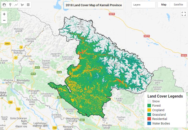
Land Cover Mapping in Google Earth Engine (Study Area Karnali Province, Nepal)
Land cover maps represent spatial information on different types (classes) of physical coverage of the Earth's surface, e.g. forests, grasslands, croplands, lakes, wetlands, snow.
Study Area and Year
Study Area is the Karnali Province of Nepal. It has an area of 24,453 km2 (9,441 sq mi). The province has occupied higher mountain land of north and mid-hills of Nepal. It contains Kubi Gangri, Changla, and Kanjiroba mountains in the north. The Shey Phoksundo National Park with Phoksundo lake is the largest national park in Nepal and Rara lake is the largest lake in Nepal which is located in Karnali Pradesh. Karnali River is the biggest river of the province which is thought to be the longest river in Nepal. The study is performed for 2018 as training data is collected in 2018.
Requirements
To generate the Landcover map in the Google Earth Engine, we need followings
-
Google Earth Engine Account
-
Ground Truth / Training data ( Spatially distributed, and different land-use class)
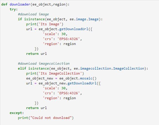
Method
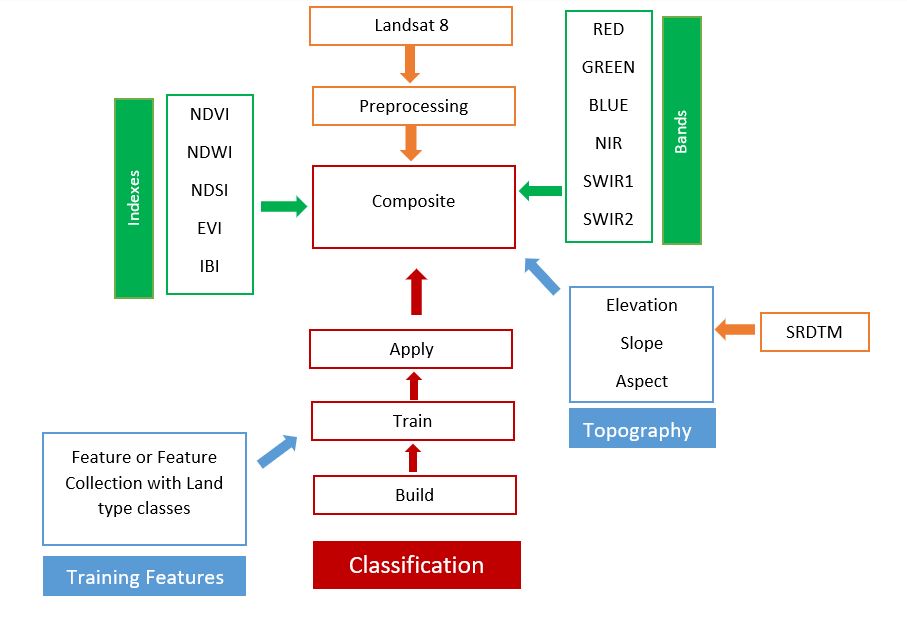
Satellite Image for the Study
Landsat 8 Imagery is used for the study. Landsat is a joint NASA/USGS program that provides the longest continuous space-based record of Earth’s land in existence. Know all the satellite data in link
//Set up bands and corresponding band names
var inBands = ee.List([1,2,3,4,5,7,6,'pixel_qa'])
var outBands = ee.List(['blue','green','red','nir','swir1','temp', 'swir2','pixel_qa'])


// Get Landsat data
var l8s = ee.ImageCollection("LANDSAT/LC08/C01/T1_SR")
    .filterDate(startDate,endDate)
    .filterBounds(studyArea)
    .select(inBands,outBands)
    .filter(ee.Filter.lt("CLOUD_COVER",10))
Bands and Indexes
For the Study prominent bands such as Red, Green, Blue, Near-Infrared, Short wave Infrared.Indexes as NDVI, NDWI, NDSI, IBI, EVI.
Know all about indexes and its important in link
function getIndexes(image){

//   Normalized Difference Vegitation Index(NDWI)
 var ndvi = image.normalizedDifference(['nir','red']).rename("ndvi");
 image = image.addBands(ndvi);


//   Normalized Difference Snow Index(NDWI)
 var ndsi = image.normalizedDifference(['green','swir1']).rename("ndsi");
 image = image.addBands(ndsi);


//   Normalized Difference Water Index(NDWI)
var ndwi = image.normalizedDifference(['nir','swir1']).rename("ndwi");
image = image.addBands(ndwi);


// add Enhanced Vegetation Indexes
var evi = image.expression('2.5 * ((NIR - RED) / (NIR + 6 * RED - 7.5 * BLUE + 1))', {
            'NIR' : image.select('nir'),
            'RED' : image.select('red'),
            'BLUE': image.select('blue') }).float();
image = image.addBands(evi.rename('evi'));


// Add Index-Based Built-Up Index (IBI)
var ibiA = image.expression('2 * SWIR1 / (SWIR1 + NIR)', {
  'SWIR1': image.select('swir1'),
  'NIR'  : image.select('nir')}).rename(['IBI_A']);

var ibiB = image.expression('(NIR / (NIR + RED)) + (GREEN / (GREEN + SWIR1))', {
  'NIR'  : image.select('nir'),
  'RED'  : image.select('red'),
  'GREEN': image.select('green'),
  'SWIR1': image.select('swir1')}).rename(['IBI_B']);

var ibiAB = ibiA.addBands(ibiB);
var ibi = ibiAB.normalizedDifference(['IBI_A', 'IBI_B']);

image = image.addBands(ibi.rename('ibi'));


return(image);


}
Topography
function getTopography(image,elevation) {

    // Calculate slope, aspect and hillshade
    var topo = ee.Algorithms.Terrain(elevation);

    // From aspect (a), calculate eastness (sin a), northness (cos a)
    var deg2rad = ee.Number(Math.PI).divide(180);
    var aspect = topo.select(['aspect']);
    var aspect_rad = aspect.multiply(deg2rad);
    var eastness = aspect_rad.sin().rename(['eastness']).float();
    var northness = aspect_rad.cos().rename(['northness']).float();

    // Add topography bands to image
    topo = topo.select(['elevation','slope','aspect']).addBands(eastness).addBands(northness);
    image = image.addBands(topo);


    return(image);
}
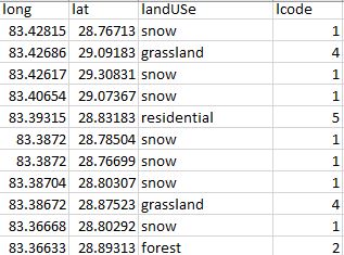
Training data
Training data is collected using Collect Earth Application and Ground Survey. Training data is categorized into
'Snow', 'Forest', 'Cropland','Grassland', 'Residential', 'Water Bodies'
Continue --- Classification
Responses

Rai
It's nice. How is the accuracy? Could you provide me GIS file? We can write a research paper.
- May 31, 2020 |
Admin
Accuracy is above 85%
- May 31, 2020 |
Feysal Hamid
It's nice
- May 31, 2020 |
Mulat
A very nice summary of the methods and requirements
- May 31, 2020 |
Srijit Sharma
Thank you so much man. You are genius. Your blog has been my life savior.
- Jul 15, 2022 |